ANOVA Calculator: Compare Process Means with a Worked Example

An ANOVA calculator helps answer a practical process-improvement question: do the average results from several groups differ beyond what their internal variation would suggest? Use one-way ANOVA for one categorical factor, such as machine, supplier or shift, and a numeric response, such as diameter, tensile strength or processing time.

This guide walks through an illustrative manufacturing example, explains the ANOVA table and shows how to turn a statistical result into a better investigation.

What does a one-way ANOVA calculator test?

One-way analysis of variance tests the null hypothesis that all population group means are equal. The alternative is that at least one differs. It is commonly used for three or more groups, although the method also works with two.

ANOVA partitions total variation into differences between group means and variation within groups. Its F statistic compares the corresponding mean squares. See the NIST overview of one-way ANOVA for the decomposition.

A significant ANOVA result identifies evidence of a difference in means. It does not identify the cause, prove that every group differs or establish that the difference matters operationally.

For a quality engineer, that distinction determines what happens next: investigate a potential machine offset, examine the production conditions or design a controlled experiment.

Worked example: do three machines produce the same average diameter?

Imagine three machines producing the same nominal 50 mm component. An engineer collects five independent parts from each machine under comparable conditions. These are synthetic teaching data, not a customer case study or evidence of an actual process improvement.

Copy the following CSV into a spreadsheet. Each row represents one part.

Machine,Diameter_mm
A,49.8
A,50.0
A,50.1
A,49.9
A,50.2
B,50.3
B,50.5
B,50.4
B,50.6
B,50.2
C,49.9
C,50.1
C,50.0
C,50.2
C,49.8

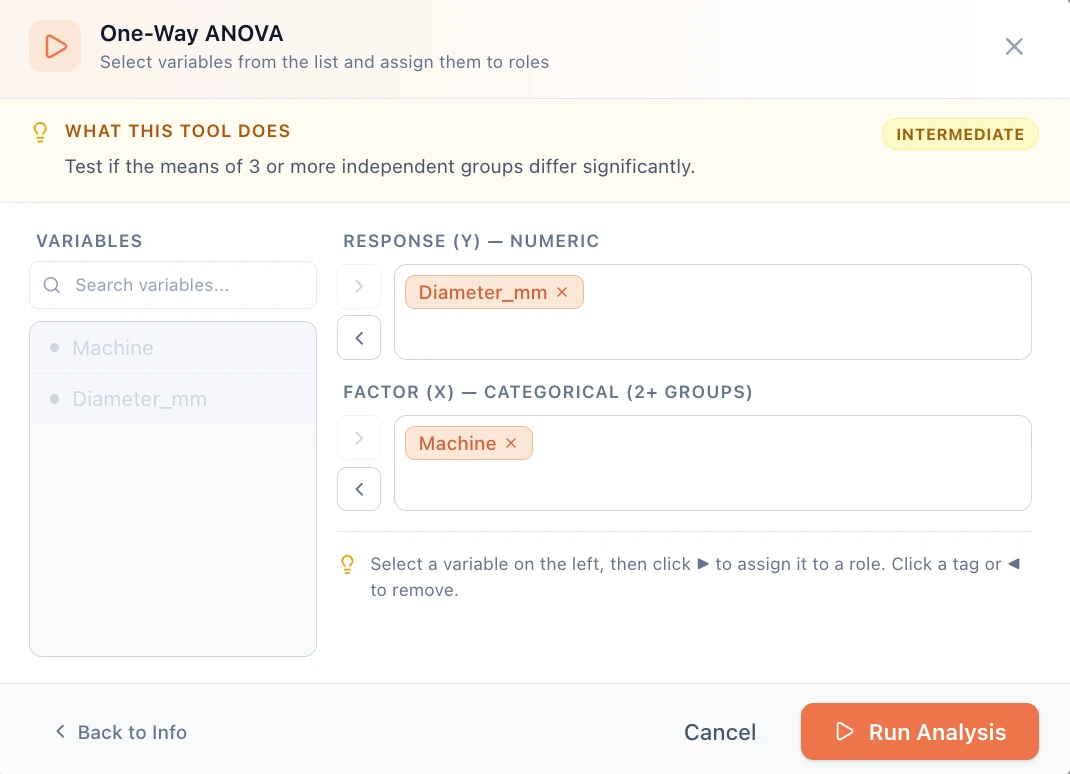
Set the numeric response to Diameter_mm and the categorical factor to Machine. Choose the significance level before examining the result; this example uses 0.05.

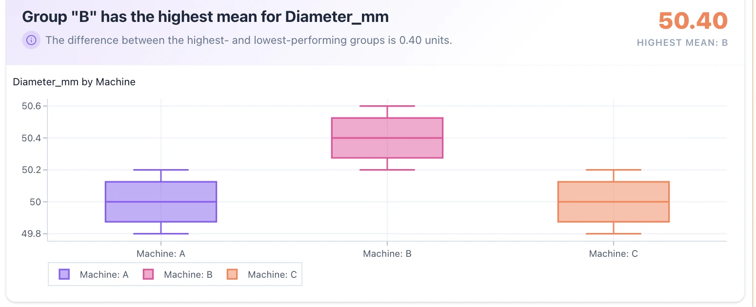
The sample means are 50.00 mm for Machine A, 50.40 mm for Machine B and 50.00 mm for Machine C. Each group has a sample standard deviation of approximately 0.1581 mm.

Expected calculation

For the classical equal-variance one-way ANOVA, the results are:

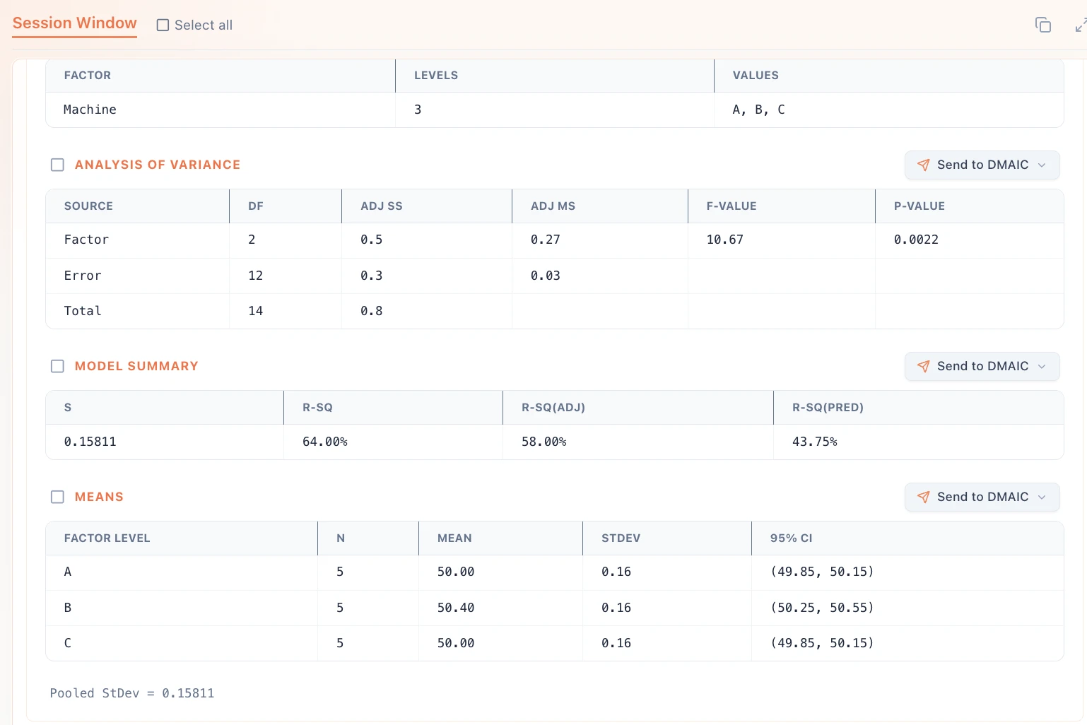
• Between machines: sum of squares = 0.533333; degrees of freedom = 2; mean square = 0.266667.
• Within machines, or error: sum of squares = 0.300000; degrees of freedom = 12; mean square = 0.025000.
• Total: sum of squares = 0.833333; degrees of freedom = 14.
• F statistic = 10.666667; p-value = approximately 0.002177.

The calculation follows F = MS_between / MS_within, or 0.266667 / 0.025000. The NIST guide to the ANOVA table explains these quantities and their degrees of freedom.

What should the engineer conclude?

Because 0.002177 is below 0.05, reject the hypothesis of equal population means, subject to the model assumptions. The data provide evidence that at least one machine's mean diameter differs.

Machine B's sample mean is 0.40 mm higher than the other two. That is an investigation lead. Before adjusting equipment, compare the difference with the engineering tolerance, measurement uncertainty and consequences for assembly or performance.

The omnibus F test alone does not establish which pairs differ. For all pairwise comparisons, an appropriate follow-up is Tukey's method under its assumptions. Its simultaneous comparisons address multiplicity; see NIST's explanation of Tukey's method. Do not treat overlapping or non-overlapping individual mean confidence intervals as a substitute for that procedure.

Five parts per machine keep this example easy to reproduce. They are not a universal sampling recommendation. Plan the sample size around the smallest meaningful difference, expected noise and required statistical power.

Check the assumptions before trusting the p-value

The classical fixed-effects model assumes independent, normally distributed errors with a common variance. These assumptions concern the errors around group means; the pooled observations need not form one normal distribution. The NIST model and assumptions provide the formal statement.

In an engineering study, translate those assumptions into collection and review checks:

• Independence: measure distinct parts and preserve collection order. Repeated measurements of the same part are not independent production observations.
• Comparable conditions: record material lot, tooling, temperature and collection time. If Machine B runs only one material lot, a machine comparison can also reflect a material difference.
• Residual behavior: examine deviations from the group means for unusual observations, changing spread and time patterns. A pooled normality test alone cannot establish model suitability.
• Measurement quality: confirm that the measurement method can resolve the difference relevant to the decision.

Identical sample standard deviations in this teaching dataset do not prove that the real process meets these assumptions. If the study structure or error behavior makes the classical model unsuitable, select a method that fits the data before interpreting its p-value.

ANOVA compares means; process improvement needs more evidence

In the example, the groups have the same sample spread but different sample means. A team could recenter Machine B and still leave its within-machine variation unchanged.

Frame the next question precisely:

• To investigate average output differences, use a suitable comparison of means.
• To investigate inconsistent output, examine spread and patterns over production order.
• To assess whether output meets specifications, evaluate capability with justified distribution and stability assumptions.
• To establish whether changing a setting improves the outcome, plan an experiment that controls competing explanations.

A lower p-value is not an improvement KPI. For this example, a useful operational question is whether a confirmed correction reduces assembly failures without increasing variation or creating another problem.

Run the example in Weibull.app

Open Weibull.app and bring the two-column dataset into your workspace. Choose One-Way ANOVA, select Diameter_mm as Response (Y) and Machine as Factor (X), then run the analysis.

Review the ANOVA table alongside the group means, sample sizes, standard deviations and mean confidence intervals. The current one-way analysis assumes equal variances. Assess assumptions separately, and use an appropriate follow-up method when pairwise conclusions are needed.

Use the worked results above to check your selections. The displayed p-value may be rounded. Preserve the study conditions and the engineering interpretation alongside the statistical output so another reviewer can assess the decision.

Frequently asked questions

What does p greater than 0.05 mean?

At a chosen significance level of 0.05, it means the test does not provide sufficient evidence to reject equal means. It does not prove equivalence. A small study may miss a difference that matters to the process.

Should I use one-way or two-way ANOVA?

One-way ANOVA addresses one factor, such as machine. When the question involves machine and material, the study needs a model that accounts for both factors and any relevant interaction. Select the analysis from the study design rather than the number of spreadsheet columns.

Does a significant result mean the process is capable?

No. This ANOVA calculation contains no specification limits. A difference among means cannot establish conformance or process capability.

Is this page an interactive ANOVA calculator?

This is a worked guide. The analysis runs inside Weibull.app, where you can apply the workflow to your own dataset.